Debt Payoff
How to Make a Debt Payoff Plan in a Spreadsheet (Google Sheets or Excel)
Build a debt payoff plan in Google Sheets or Excel: the columns you need, how to calculate monthly interest, roll payments forward, and estimate a debt-free date.
On this page
- What your plan needs to answer
- Step 1: Gather the numbers
- Step 2: Build the debt list
- Step 3: Pick your extra amount
- Step 4: Choose an order
- Step 5: Build the month-by-month schedule
- Step 6: Find each payoff month
- Step 7: Add progress tracking
- Common spreadsheet mistakes
- Keep the plan realistic
- The shortcut
- When to get help
- A monthly routine that works
- A sample layout you can copy
A debt payoff plan turns a vague goal ("get out of debt") into a list of numbers you can act on every month: which debt to pay extra, how much, and roughly when each one will be gone. A spreadsheet is the perfect tool because it does the repetitive interest math for you. This guide shows how to build one in Google Sheets or Excel from a blank page.
What your plan needs to answer
- How much do I owe in total, and at what rates?
- What's the minimum I must pay each month?
- How much extra can I add?
- Which debt gets the extra first?
- When will each debt be paid off, and roughly how much interest will I pay?
Step 1: Gather the numbers
For each debt, collect from your statement or online account:
- Name (e.g., "Visa", "Car loan")
- Current balance
- Interest rate (APR)
- Minimum monthly payment
- Due date
Be honest and complete. Include medical bills, buy-now-pay-later plans, and money owed to family if you intend to repay it.
Step 2: Build the debt list
On a tab called Debts, make a table with the columns above. Add a total row at the bottom for balance and minimum payments using =SUM(). That total minimum is the floor: you must pay at least that each month.
Step 3: Pick your extra amount
In a separate cell, enter the extra amount you can add every month beyond the minimums. Look at your budget for a realistic number. If you're paid biweekly, a paycheck budget will show how much leftover you really have. Your total monthly debt budget is the total minimum plus the extra.
Step 4: Choose an order
Add a "Priority" column. For the snowball, rank by smallest balance. For the avalanche, rank by highest APR. Not sure which? Read our snowball vs. avalanche worked example.
Step 5: Build the month-by-month schedule
On a new tab called Schedule, create one block of columns per debt and one row per month. For each debt in each month:
- Starting balance: last month's ending balance.
- Interest: starting balance × APR ÷ 12. In a cell:
=B2*$APR/12. - Payment: the minimum, or more if this is the priority debt (see below), but never more than the balance plus interest. Use
=MIN(minimum, balance+interest)as a base. - Ending balance: starting balance + interest − payment.
The priority debt receives whatever is left of the total monthly debt budget after all the minimums are paid. When a debt's balance hits zero, its minimum is no longer needed, so the leftover grows automatically. That's the "rollover" that speeds everything up.
This logic is the trickiest part to write by hand, because the extra money must flow to whichever debt is currently first in line. One workable approach is a helper column that calculates "money left after minimums" each month and assigns it in priority order using MIN() so no debt is overpaid.
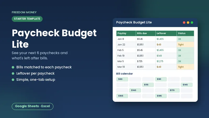
Free: Paycheck Budget Lite
A simple starter spreadsheet for Google Sheets or Excel. List your take-home pay and bills and see what each paycheck has left. Free, instant download.
Download the free templateStep 6: Find each payoff month
Add a summary row that finds the first month where each debt's ending balance is zero, using something like =INDEX(month_column, MATCH(TRUE, balance_column<=0, 0)) (entered as an array formula in Excel, or wrapped with ARRAYFORMULA in Google Sheets if needed). Total the interest column for each debt to see estimated interest paid.
Step 7: Add progress tracking
Plans are more motivating when you can see progress. Add:
- A "Paid so far" column that compares the original total with today's total.
- A simple progress bar using
=SPARKLINE()in Google Sheets, or a data bar in Excel's conditional formatting. - A row for actual payments so you can compare plan vs. reality.
Common spreadsheet mistakes
- Using the yearly rate as monthly. Divide APR by 12 for monthly interest.
- Forgetting the rollover. If a paid-off debt's minimum doesn't move to the next debt, the plan is too slow.
- Overpaying the last month. Cap payments at balance plus interest.
- Never updating balances. Once a month, replace the starting balances with the real numbers from your statements. Real interest can differ slightly due to daily compounding and posting dates.
Keep the plan realistic
Interest on credit cards is usually calculated on daily balances, and rates can change. A spreadsheet plan is an estimate, not a promise. That's fine. Its job is to show you direction and order, and to keep you consistent. Update it monthly and the estimate gets more accurate as balances fall.
The shortcut
If you'd rather not build the rollover logic, our Debt Payoff Tracker has it done: list your debts, choose snowball or avalanche, and see an estimated payoff month for each debt, total interest, and a side-by-side comparison of both strategies. It works in Google Sheets, Excel, and LibreOffice.
When to get help
If minimum payments are more than you can cover, a spreadsheet won't fix that on its own. The CFPB's free resources at consumerfinance.gov explain options like nonprofit credit counseling and what to watch out for with debt relief offers.
A monthly routine that works
- On statement day, update each balance.
- Confirm all minimums are scheduled.
- Send the extra to the priority debt.
- Check off any paid-off debt and celebrate a little.
- Glance at the estimated debt-free date. Watching it move earlier is the reward.
A sample layout you can copy
| Month | Card A start | Card A interest | Card A paid | Card A end | Extra left for next debt |
|---|---|---|---|---|---|
| 1 | $1,000.00 | $20.00 | $345.00 | $675.00 | $0 |
| 2 | $675.00 | $13.50 | $345.00 | $343.50 | $0 |
| 3 | $343.50 | $6.87 | $345.00 | $5.37 | $0 |
| 4 | $5.37 | $0.11 | $5.48 | $0.00 | $339.52 |
In this illustration, Card A has a $1,000 balance at 24% APR and receives $345 a month (a $45 minimum plus $300 extra). In month 4 it only needs $5.48, so the remaining $339.52 flows to the next debt that same month. That's the rollover in action, and it's why the last debts on your list fall much faster than the first one.
Frequently asked questions
How do I calculate monthly interest on a debt?
Divide the APR by 12 and multiply by the balance. For example, a $1,000 balance at 24% APR accrues about $20 in a month.
What is a debt rollover?
When a debt is paid off, you add its old payment to the next debt on your list instead of spending it, so payments grow over time.
Is a spreadsheet payoff date exact?
No, it's an estimate. Daily interest and posting dates make real numbers differ slightly, so update balances monthly.
This guide is general educational information, not financial, tax, legal, or insurance advice. Examples are illustrations, not predictions. See our disclaimer.